Aug 28, 2022

Anomaly Detection with a Custom MAD Estimator in scikit-learn

statistics anomaly detection scikit-learn

When you need a lightweight anomaly detector, the Mean Absolute Deviation (MAD) is an appealing option: it is robust to outliers, easy to explain, and fast to compute. The catch is that scikit-learn does not ship a ready-made estimator for it. In this walkthrough we will fill that gap by implementing a reusable MAD-based detector that integrates cleanly with the scikit-learn API, pipelines, and model selection tools.

Why MAD for anomaly detection?

The MAD measures how far the values in a distribution deviate from a robust center. We compute it in three steps:

Estimate the center with the median.
Measure the absolute deviations from that median.
Take the median of those deviations and scale it so it is comparable with the standard deviation.

A point is flagged as an anomaly when its deviation exceeds a multiple of the scaled MAD. Because the median is insensitive to extreme values, the detector can resist the very outliers it is tasked with finding.

Implementing a scikit-learn compatible estimator

Our goal is to produce an object that behaves like any other scikit-learn estimator. That means supporting the familiar methods fit, predict, decision_function, and fit_predict, plus parameter introspection for grid searches. We can achieve this by inheriting from BaseEstimator and OutlierMixin.

import numpy as np
from sklearn.base import BaseEstimator, OutlierMixin
from sklearn.utils.validation import check_array

class MadOutlierDetector(BaseEstimator, OutlierMixin):
    """Flag points whose median-based z-score exceeds a threshold."""

    def __init__(self, threshold=2.5):
        self.threshold = threshold

    def fit(self, X, y=None):
        X = check_array(X)
        # Median along each feature dimension for robustness to outliers.
        self.location_ = np.atleast_1d(np.median(X, axis=0))
        # Median absolute deviation with scaling factor for normal consistency.
        mad = np.median(np.abs(X - self.location_), axis=0)
        self.scale_ = np.atleast_1d(1.4826 * mad)
        # Avoid division by zero for constant features.
        self.scale_[self.scale_ == 0] = 1e-9
        return self

    def decision_function(self, X):
        X = check_array(X)
        deviations = np.abs(X - self.location_)
        mad_scores = deviations / self.scale_
        # Reduce to 1D score per sample by taking the max deviation across features.
        return mad_scores.max(axis=1)

    def predict(self, X):
        scores = self.decision_function(X)
        return np.where(scores > self.threshold, -1, 1)

    def partial_fit(self, X, y=None):
        raise NotImplementedError('MAD detector does not support online updates.')

Key design choices:

threshold controls how aggressive the detector is. Values around 2–3 work well for most datasets, with lower values being more sensitive to outliers.
By using decision_function we remain compatible with scikit-learn tooling that expects anomaly scores where higher means “more anomalous”.
The estimator returns labels 1 for normal points and -1 for anomalies, matching OutlierMixin conventions.

Using the detector on synthetic data

Let us see the estimator in action on a realistic one-dimensional dataset that simulates a mean shift scenario with clear anomalies. This type of data is common in time series monitoring where you might see a sudden change in the underlying process. We compare the predictions against scikit-learn’s IsolationForest to highlight how you might blend fast statistical checks with heavier algorithms.

import matplotlib.pyplot as plt
from sklearn.ensemble import IsolationForest
from sklearn.pipeline import Pipeline
from sklearn.preprocessing import StandardScaler

# Generate data: mean shift scenario with clear anomalies
rng = np.random.default_rng(42)

# First phase: tight cluster around -1
phase1 = rng.normal(loc=-1, scale=0.2, size=200)

# Second phase: mean shift to +2
phase2 = rng.normal(loc=2, scale=0.2, size=200)

# Third phase: high variance with some extreme outliers
phase3 = rng.normal(loc=0, scale=2, size=100)
# Add some extreme outliers
extreme_outliers = rng.normal(loc=-8, scale=1, size=20)

X = np.concatenate([phase1, phase2, phase3, extreme_outliers]).reshape(-1, 1)

mad_detector = MadOutlierDetector(threshold=2.5)
isolation_forest = IsolationForest(n_estimators=200, contamination=0.1, random_state=42)

# MAD detector works better without standardization for this synthetic data
# Isolation Forest still benefits from standardization
mad_pipeline = Pipeline([('detector', mad_detector)])
iso_pipeline = Pipeline([
    ('scaler', StandardScaler()),
    ('detector', isolation_forest)
])

mad_labels = mad_pipeline.fit_predict(X)
iso_labels = iso_pipeline.fit_predict(X)

mad_scores = mad_pipeline[-1].decision_function(X)
iso_scores = -iso_pipeline[-1].score_samples(iso_pipeline[0].transform(X))  # higher = more anomalous

The MAD detector works directly on the raw data, while the Isolation Forest benefits from standardization. This approach allows the MAD detector to leverage the natural scale of the data for better outlier detection.

Interpreting the output

With the labels and scores in hand we can inspect the flagged points.

anomaly_idx = np.where(mad_labels == -1)[0]
# Calculate bounds directly since no scaler is used
lower = (mad_pipeline[-1].location_[0] - mad_pipeline[-1].threshold * mad_pipeline[-1].scale_[0])
upper = (mad_pipeline[-1].location_[0] + mad_pipeline[-1].threshold * mad_pipeline[-1].scale_[0])

# Debug information
print(f"Number of anomalies detected: {len(anomaly_idx)}")
print(f"Location (median): {mad_pipeline[-1].location_[0]:.3f}")
print(f"Scale (MAD): {mad_pipeline[-1].scale_[0]:.3f}")
print(f"Threshold: {mad_pipeline[-1].threshold}")
print(f"Bounds: [{lower:.3f}, {upper:.3f}]")

plt.figure(figsize=(10, 4))
plt.scatter(np.arange(X.size), X[:, 0], c='lightgray', label='observations')
plt.scatter(anomaly_idx, X[anomaly_idx, 0], c='tab:red', label='MAD anomalies')
plt.axhline(upper, color='tab:blue', linestyle='--', linewidth=1, label='threshold bounds')
plt.axhline(lower, color='tab:blue', linestyle='--', linewidth=1)
plt.title('MAD detector vs. synthetic data')
plt.legend()
plt.show()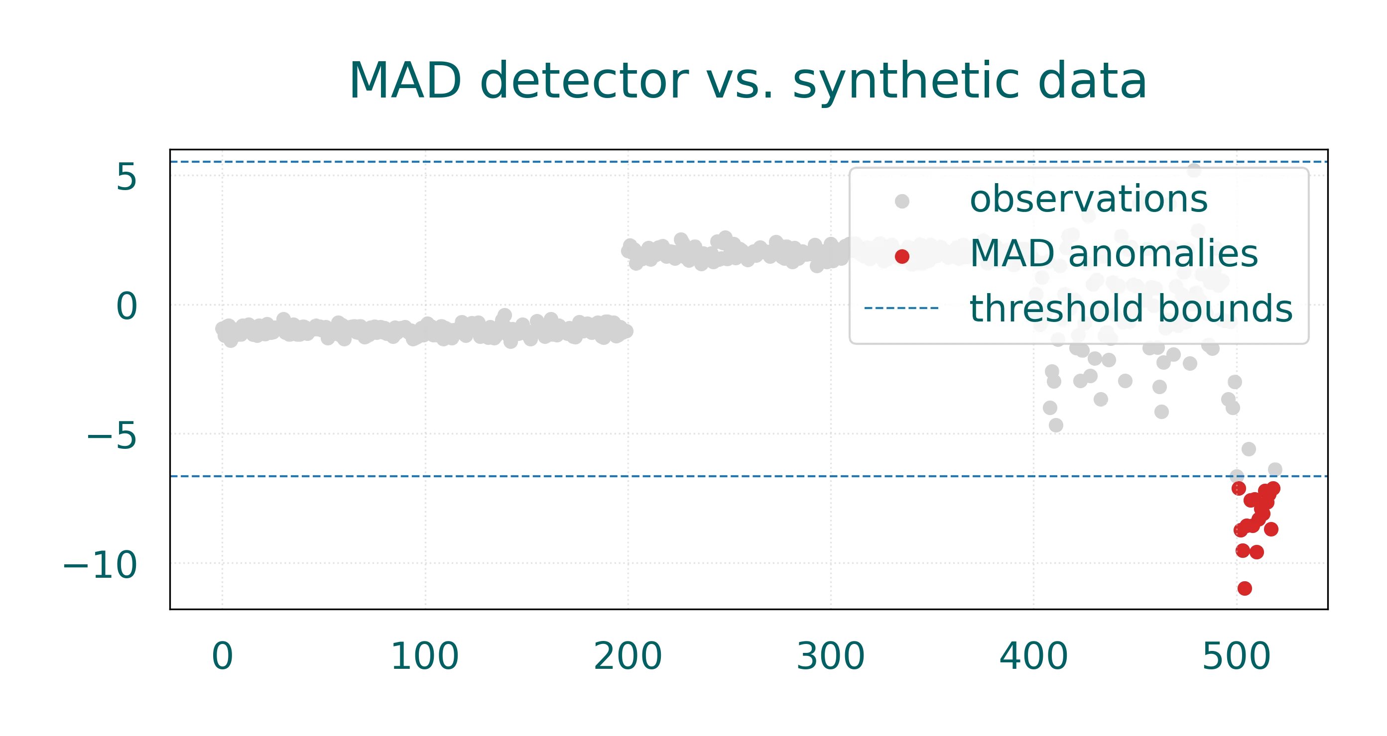

MAD detector vs. synthetic data

On this dataset the MAD detector effectively identifies the extreme outliers in the third phase of our synthetic data. The detector’s robustness comes from using the median as the central location estimate, which is less affected by outliers than the mean. The debug output helps us understand the detector’s behavior: it shows the median location, the MAD scale, and the threshold bounds used for classification.

Because its calculations are closed-form, the MAD detector scales to millions of rows and can serve as a fast preprocessing filter or a nice baseline. When the data is high-dimensional or highly skewed, a model such as IsolationForest or LocalOutlierFactor may perform better, but you can still use MAD as an inexpensive first pass.

Extending the estimator

The custom class is a starting point that you can adapt to your needs:

Feature-wise vs. joint deviations: For correlated features you might replace the max aggregation with a Mahalanobis-type distance computed from robust covariance estimates.
Multi-dimensional thresholds: Set different threshold values per feature or make it a parameter learned from validation data.
Pipeline integration: Because the estimator follows scikit-learn’s API, you can combine it with transformers, nest it inside OneVsRestClassifier, or tune threshold via GridSearchCV.

Takeaways

Building a MAD-based anomaly detector in scikit-learn takes only a few lines of code, yet yields a tool that is fast, interpretable, and production-friendly. By wrapping the core statistic in a custom estimator you gain access to the full scikit-learn ecosystem (pipelines, cross-validation, model persistence, etc.) while keeping the mathematical simplicity that makes MAD attractive for anomaly detection.