Churn is not a single number; it’s a survival process. Treating it with a Bayesian model gives you retention curves with honest uncertainty, parameters you can interpret, and a natural way to update beliefs as new data arrives.

---

Churn as a metric

Most dashboards reduce churn to something like “we lost 5% of customers last month.” That’s workable for quick checks, but incomplete:

• It ignores customer age (new vs. seasoned customers don’t behave the same).
• It collapses a time-varying process into one ratio.
• It hides uncertainty as if churn is known precisely.

If we want decisions (budgets, roadmap, lifecycle nudges) to be proportional to reality, we need a model that evolves over time and carries its own uncertainty.

Churn as a distribution

Think of each customer as having a lifetime $(T)$: the time from start to churn. Some haven’t churned yet; they’re right-censored (we only know $T >$ something).

Survival analysis gives us three fundamental pieces:

• Survival $S(t) = P(T>t)$ (retention).
• Density $f(t)$ (how lifetimes are distributed).
• Hazard $h(t) = \frac{f(t)}{S(t)}$ (the instantaneous risk of churn at time $t$, given survival so far).

Real businesses often have time-varying hazard: early drop-offs (onboarding friction) followed by a long tail of loyalists.

The Bayesian view

Instead of estimating a few point values, we infer distributions over parameters:

• Priors encode reasonable assumptions (e.g., “we expect more churn early on”).
• Posterior combines priors with data to yield updated beliefs.
• Credible intervals (e.g., 95%) say: given our model and data, there’s a 95% probability the parameter/curve lies in this range.

This buys us three things:

1. No false precision since uncertainty is explicit.
2. Continuous learning via just updating with new data.
3. Graceful handling of censoring and small samples.

Building a simple Bayesian churn model

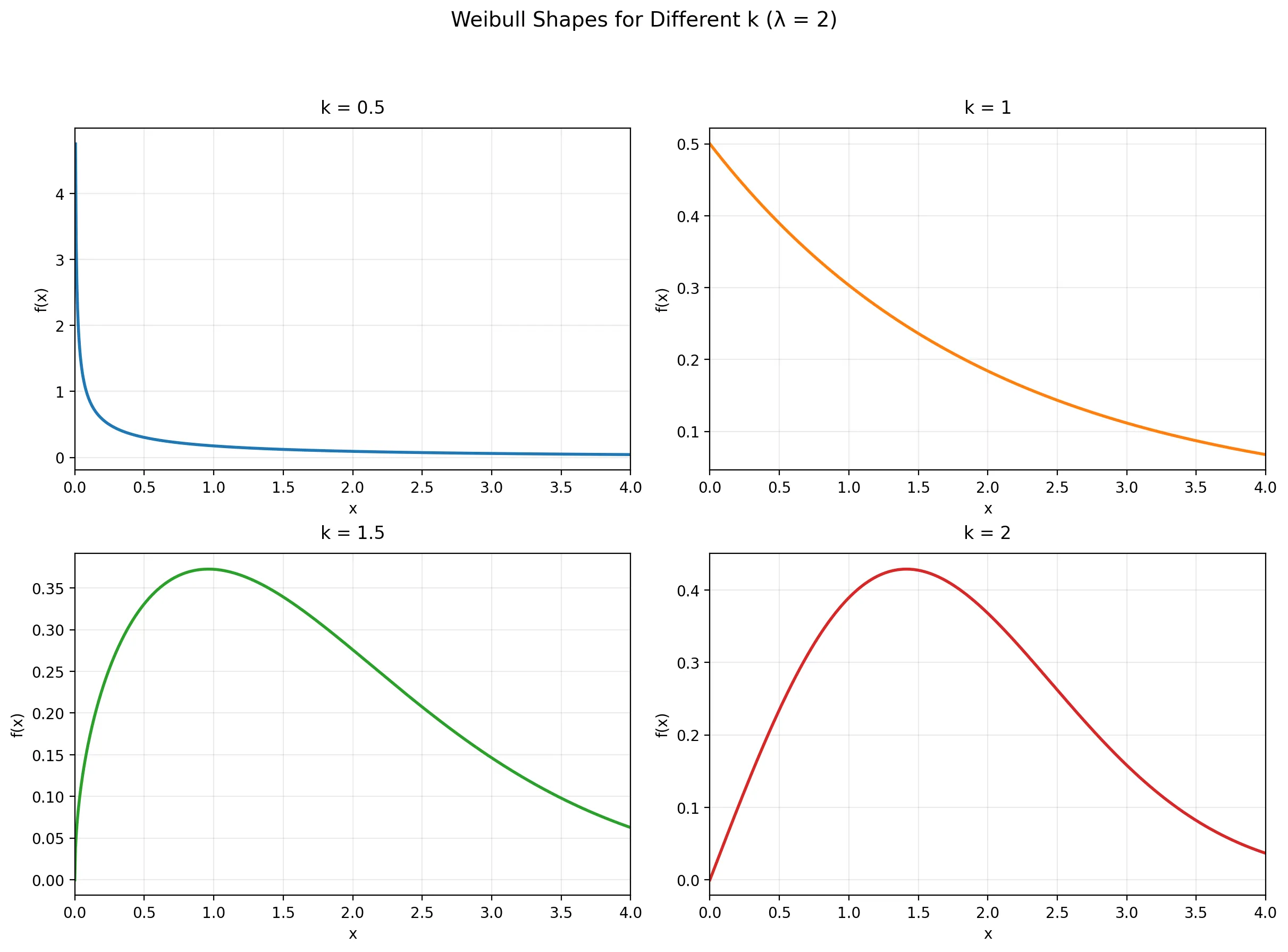
A pragmatic starting point is a Weibull lifetime model:

• Shape ($k$) determines how risk evolves.

  • ($k < 1$): risk decreases over time (strong early churn).
  • ($k=1$): constant risk (exponential).
  • ($k>1$): risk increases (wear-out or fatigue).

• Scale ($\lambda$) is the time scale (roughly, the horizontal stretch of the curve).

We model observed durations (some censored) using a Weibull likelihood, then infer ($k$) and ($\lambda$).

In python we can use the PyMC library to build this model and sample from the posterior distribution.

durations = df["duration"].values.astype(float)
events = df["event"].values.astype(int)

# right-censoring
upper = np.where(
    events == 1, np.inf, durations
)

with pm.Model() as model:
    # Priors (log-normal keep parameters positive)

    # shape (k or alpha) keep it flexible
    k = pm.LogNormal("k", mu=0.0, sigma=0.5)

    # scale (lambda or beta)
    lam = pm.LogNormal("lam", mu=np.log(6.0), sigma=1.0)

    # Right-censored likelihood
    obs = pm.Censored(
        "obs",
        pm.Weibull.dist(
            alpha=k, beta=lam
        ),  # alpha=shape=k, beta=scale=lam
        upper=upper,
        observed=durations,
    )

    # sample from the posterior distribution
    idata = pm.sample(
        draws=draws,
        tune=tune,
        chains=chains,
        target_accept=target_accept,
        random_seed=seed,
        progressbar=True,
    )

Understanding the model

From the posterior draws of $k$ and $\lambda$, we can:

• Plot retention curves $S(t)$ with credible bands (honest uncertainty).
• Compute interpretable summaries, e.g. retention at 6 months with a 95% credible interval.
• Compare the dashboard’s single churn rate with a posterior predictive view that flexes over time.

Learning in real time

Because the posterior is a probability distribution, updating is straightforward: append new data (new cohorts), refit, and your uncertainty tightens or shifts. You can also add hierarchical structure (e.g., plans, channels or regions) so information partially pools—stabilizing sparse groups without washing out real differences.

Why this matters beyond metrics

• Decision quality: Budgeting and lifecycle timing depend on how uncertain you are.
• Culture: It’s healthier to be honestly uncertain than falsely precise.
• Mindset: Bayesian modeling is a habit of thought—treat beliefs as revisable, and let the data move you.

Conclusion

Churn isn’t a static KPI to be reported once and forgotten, it’s a dynamic survival process that unfolds over time. By framing it as a distribution rather than a single percentage, we gain access to retention curves that evolve, hazard functions that reveal when customers are most at risk, and honest uncertainty bounds that inform better decisions. A Bayesian Weibull model offers a pragmatic starting point since it’s simple enough to interpret, flexible enough to capture real-world patterns like early drop-offs or long-tail loyalty, and naturally extensible to hierarchical structures when you need to pool information across segments. The real payoff isn’t just better charts, it’s a shift in how you think about uncertainty. Instead of pretending to know churn precisely, you can acknowledge what you don’t know, update your beliefs as new data arrives, and make decisions proportional to that uncertainty. Whether you’re setting retention budgets, timing lifecycle interventions, or simply building a healthier data culture, treating churn as a Bayesian survival process gives you the tools to be both rigorous and honest.