Dec 17, 2023

Multi-Armed Bandits for Optimizing Experiments

by Juan Gesino

statistics causal inference a/b testing

---

The problem with classic A/B tests

So you’re running an A/B test on three email subject lines. You know the drill: split your traffic three ways, wait for the data to pile up, run your tests, pick a winner. But here’s the issue: while you’re learning, you’re deliberately showing the bad variants to tons of users. You might suspect variant B is better after day two, but you keep sending traffic to the losers anyway because “we need statistical significance.”

There’s a better way.

The multi-armed bandit

Instead of using a fixed split, what if our system could learn while allocating traffic? Start exploring all the options, but gradually shift more users toward whatever’s working. That’s the bandit approach. The name comes from slot machines (the “arms” in casino slang). Picture yourself in front of a row of slot machines, each with its own unknown payout. You want to walk away with as much money as possible, not just a report on which machine is objectively the best. We’re going to build this from scratch, no heavy math, just code and intuition.

A step back

Let me break down the vocabulary real quick:

Arms are your options at each step. Could be subject lines, UI variants, ad creatives, WhatsApp templates (see Bayesian A/B Testing WhatsApp Messages), whatever you’re testing.

Reward is the outcome you care about. Did they click? Did they sign up? How much revenue came through?

The goal is to maximize your total reward over time, not just identify “the winner” at the end. That’s the key shift from traditional A/B testing.

And here’s the core concept that makes this interesting: you need to explore (try different arms to learn about them) while also exploiting (picking what currently looks best). Every time a user shows up, the algorithm has to decide: which arm should I show them, given everything I’ve seen so far?

Building a toy world

Okay, time to write some code. We’re going to simulate a simple environment where each arm has its own click-through rate (CTR). The algorithm won’t know these true rates, it’ll just see 0s and 1s (click or no click). But we’ll know them so we can see how well the algorithm learns.

import numpy as np
import matplotlib.pyplot as plt


np.random.seed(42)

# Three arms with different probabilities
true_ctr = np.array([0.05, 0.08, 0.12])
n_arms = len(true_ctr)

def pull_arm(arm, true_ctr=true_ctr):
    """
    Simulate pulling an arm.
    Return 1 with probability true_ctr[arm], else 0.
    """
    return int(np.random.rand() < true_ctr[arm])

Each arm is basically a subject line with its own CTR. The world randomly returns 0 or 1 based on the true rate, and our algorithms just see these outcomes roll in.

We start with a baseline

Before we get clever, let’s see what happens when you just pick randomly. This is basically what a traditional A/B/n test does with its fixed equal split.

T = 10_000  # number of users

chosen_arms = np.zeros(T, dtype=int)
rewards = np.zeros(T, dtype=int)

for t in range(T):
    arm = np.random.randint(n_arms)  # uniformly random choice
    reward = pull_arm(arm)
    chosen_arms[t] = arm
    rewards[t] = reward

# tracking performance
cumulative_reward = np.cumsum(rewards)
average_reward = cumulative_reward / (np.arange(T) + 1)

Let’s visualize what’s happening:

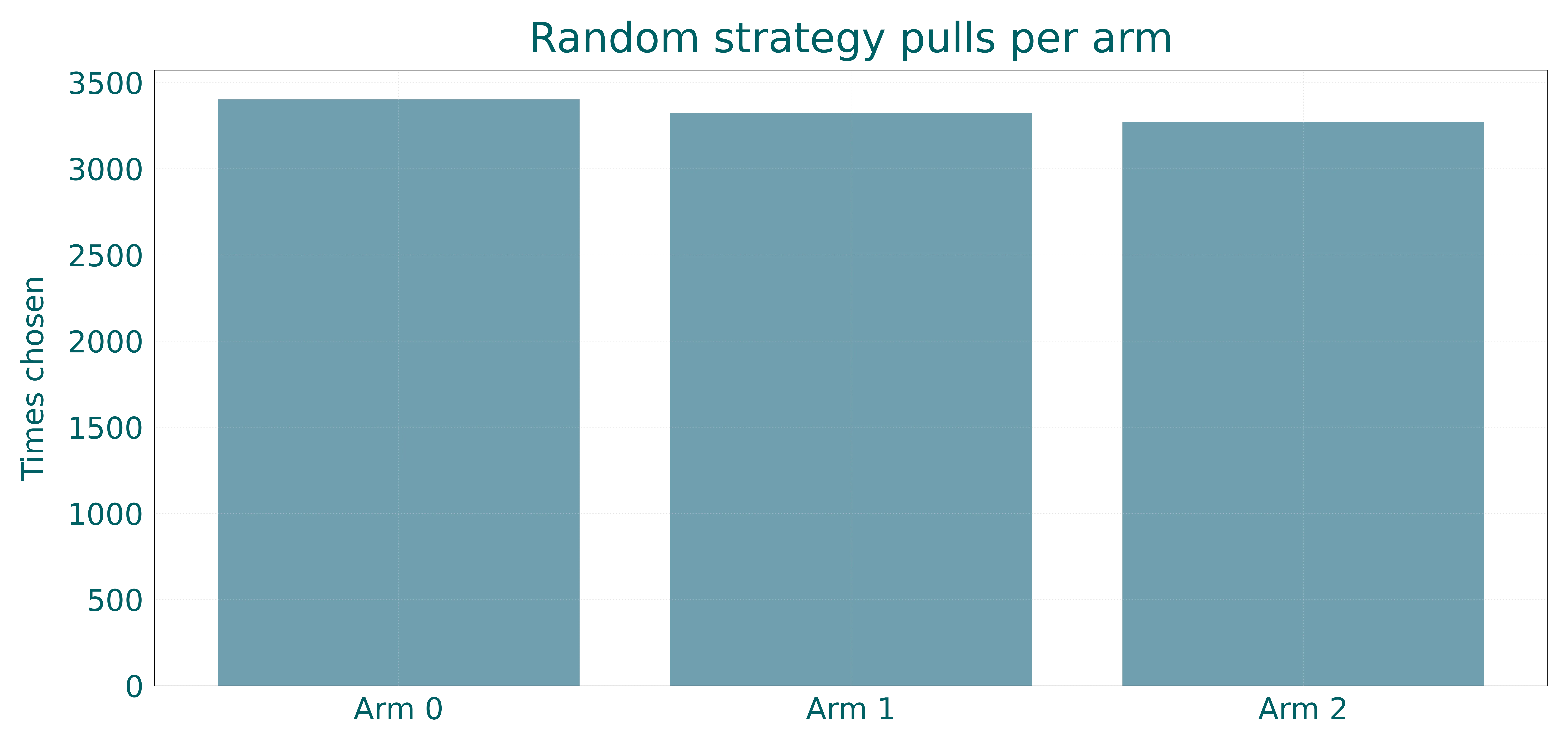
Unsurprisingly, each arm gets roughly equal traffic. That’s exactly what we’d expect from a fixed-split test.

Now let’s look at the cumulative reward over time:

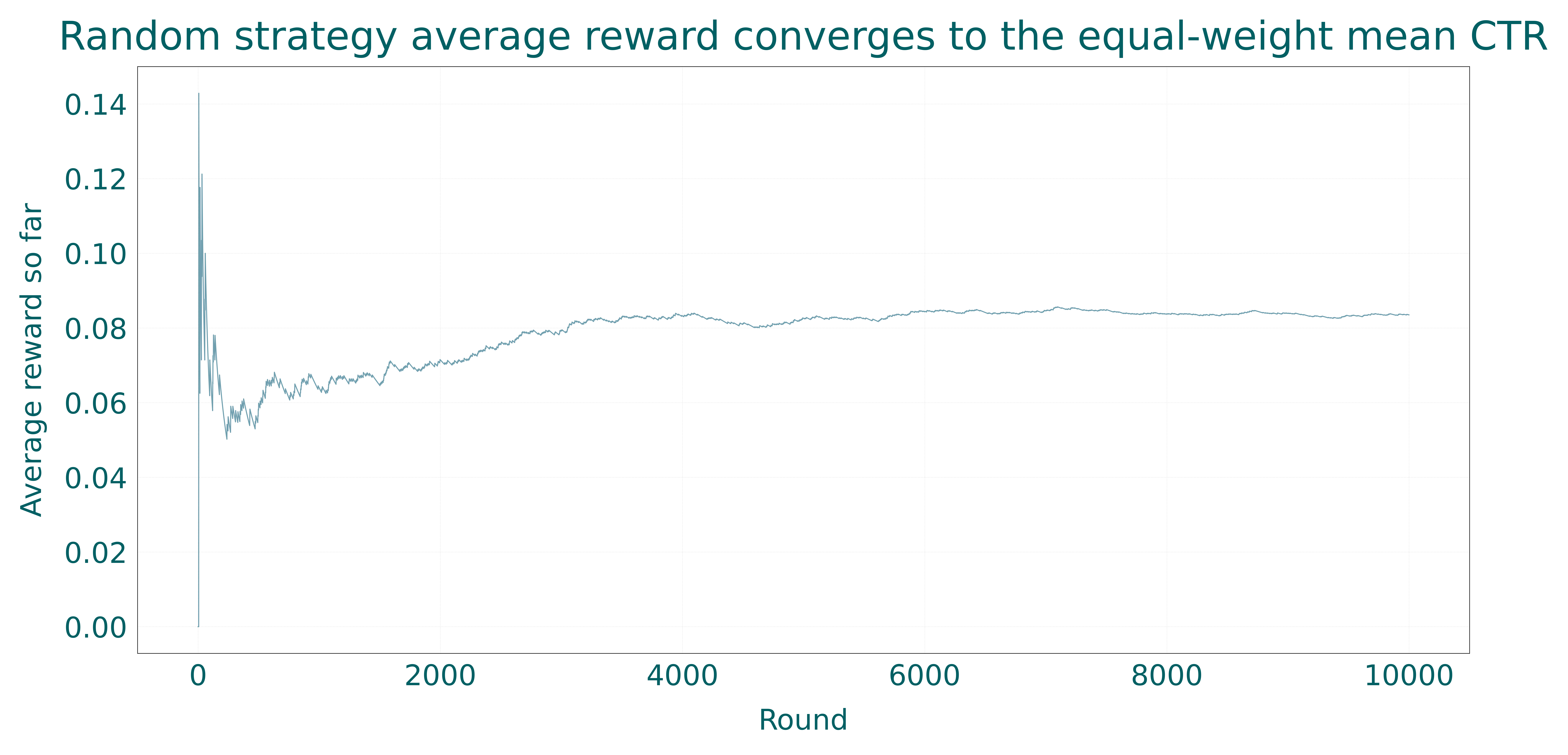
The average reward converges to about 0.083, which is the equal-weight average of our three CTRs. That’s fine for learning, but we’re definitely leaving clicks/money on the table by treating all arms equally.

We can do better

Here’s the idea: we’ll keep running estimates of each arm’s CTR. Then, every time a user shows up, we flip a weighted coin:

• With probability ε (say, 0.1): we explore (pick a random arm to keep learning)
• With probability 1 - ε (so, 0.9): we exploit (pick whichever arm currently has the highest estimated CTR)

This way we’re mostly going with what looks good, but we still occasionally check in on the other options.

eps = 0.1
T = 10_000

counts_eps = np.zeros(n_arms, dtype=int)
value_estimates = np.zeros(n_arms, dtype=float)

chosen_arms_eps = np.zeros(T, dtype=int)
rewards_eps = np.zeros(T, dtype=int)

for t in range(T):
    if np.random.rand() < eps:
        # explore: pick a random arm
        arm = np.random.randint(n_arms)
    else:
        # exploit: pick arm with highest estimated CTR
        arm = np.argmax(value_estimates)

    reward = pull_arm(arm)

    # incremental mean update for the chosen arm
    counts_eps[arm] += 1
    value_estimates[arm] += (reward - value_estimates[arm]) / counts_eps[arm]

    chosen_arms_eps[t] = arm
    rewards_eps[t] = reward

# tracking performance
cumulative_reward_eps = np.cumsum(rewards_eps)
average_reward_eps = cumulative_reward_eps / (np.arange(T) + 1)

So where does the traffic actually go?

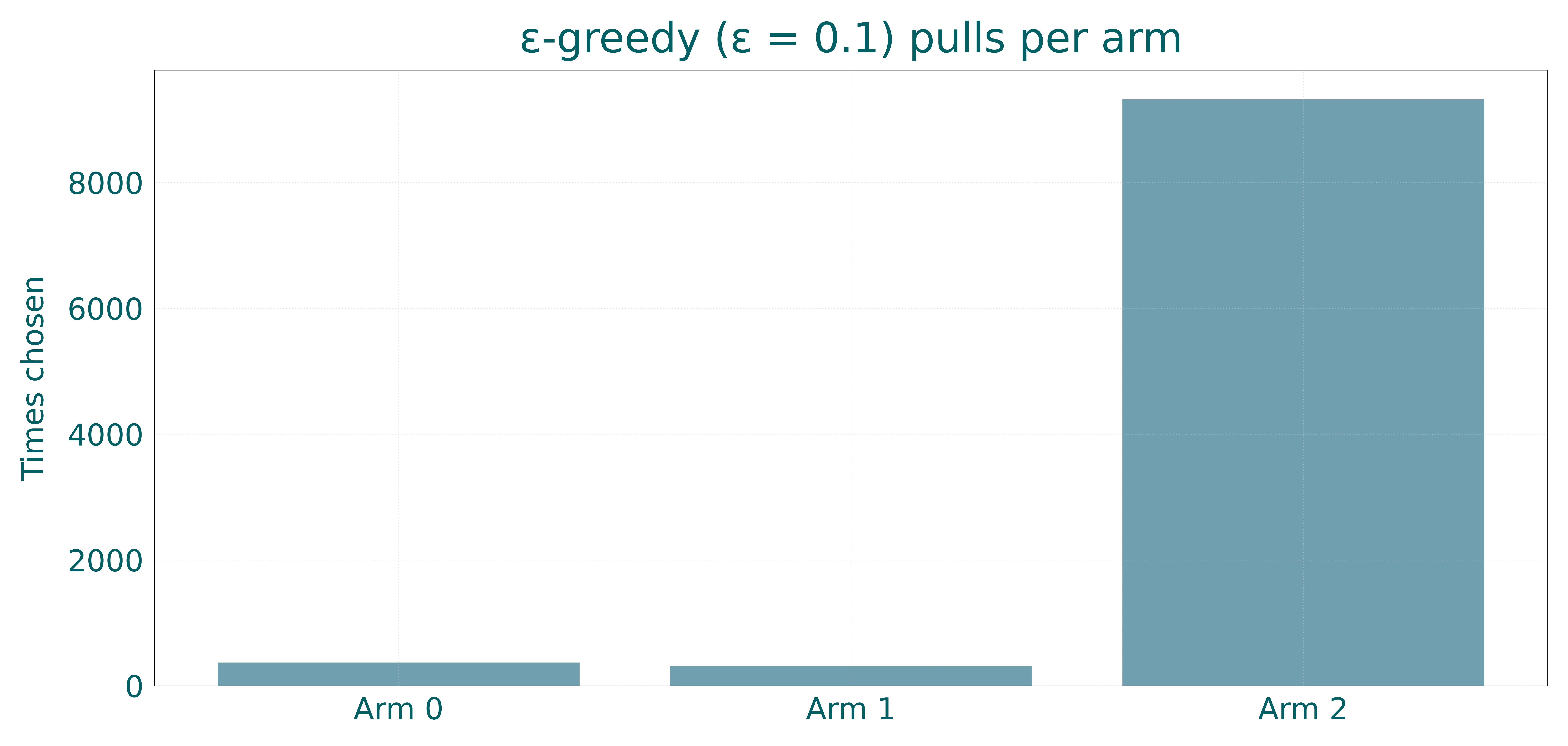
Now we’re talking! The best arm gets most of the traffic, and the worst arm barely gets shown. This is the algorithm learning and exploiting that knowledge.

Here’s another way to see it, let’s track what percentage of traffic goes to the best arm over time:

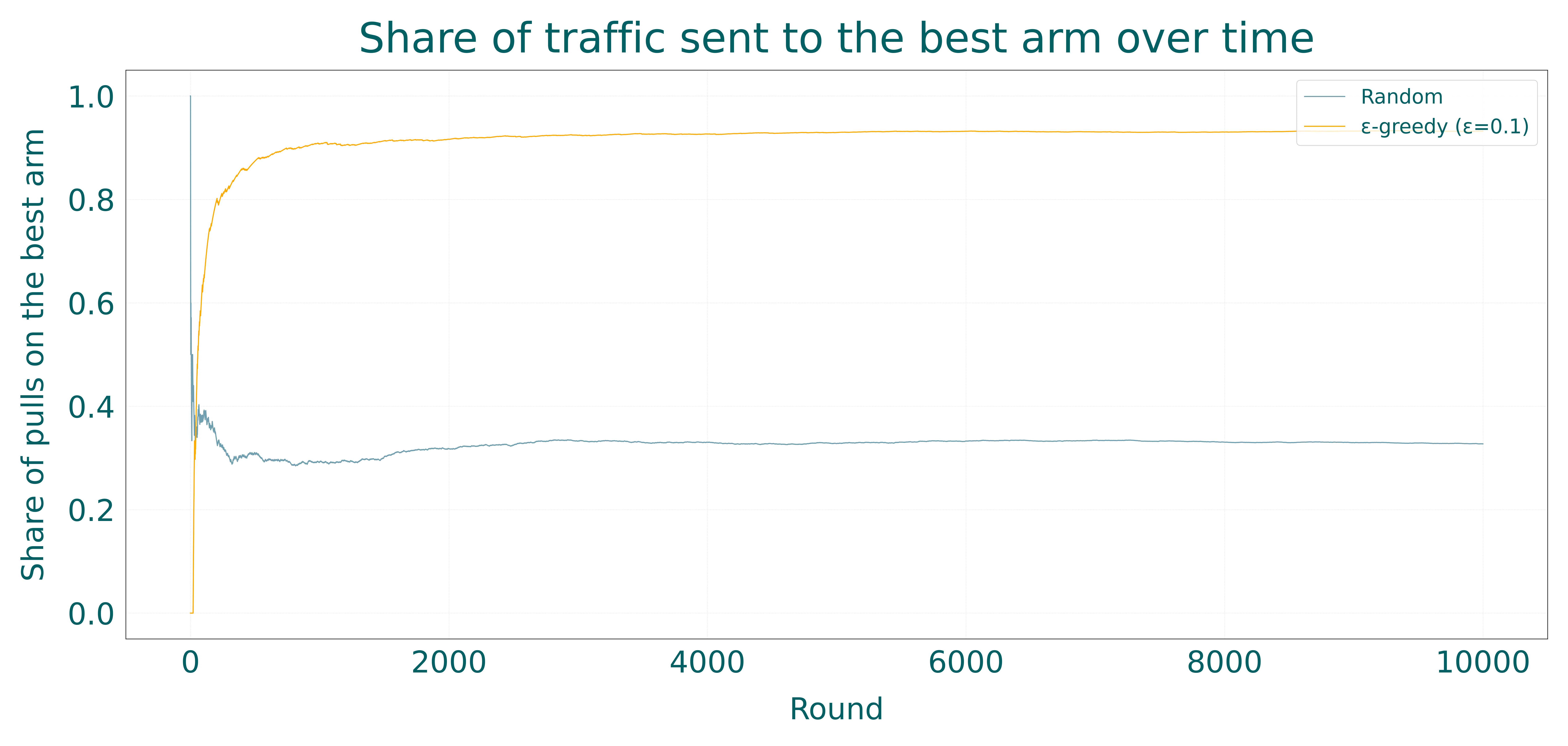
The random strategy hovers around 1/3 (as expected), while ε-greedy climbs well above that as it learns which arm is best.

You think that’s impressive? Let’s look at the cumulative reward:

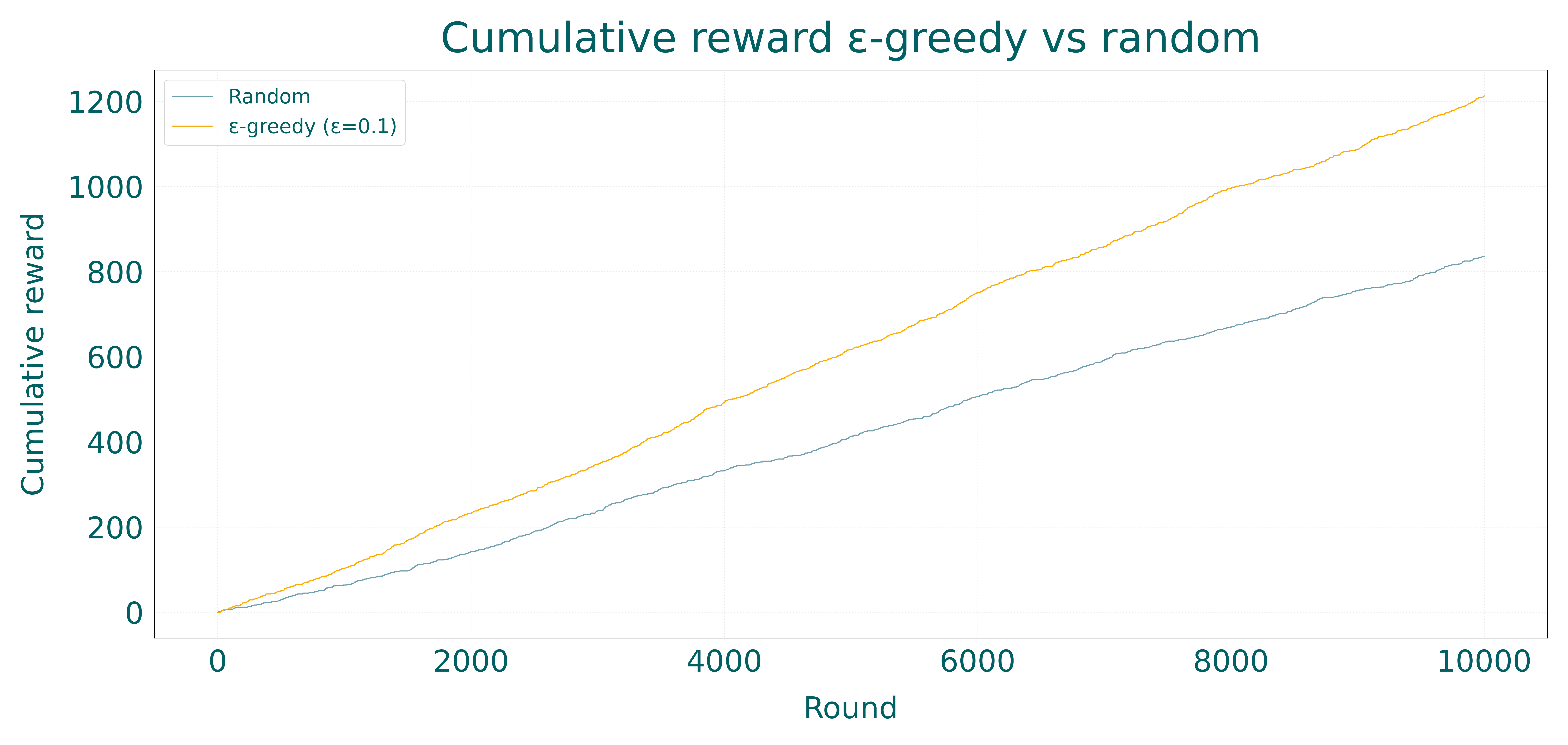
The ε-greedy curve sits above the random curve. Same amount of traffic, more total clicks. That’s the entire bandit value proposition in one picture.

And just to close the loop, let’s check how good our CTR estimates are:

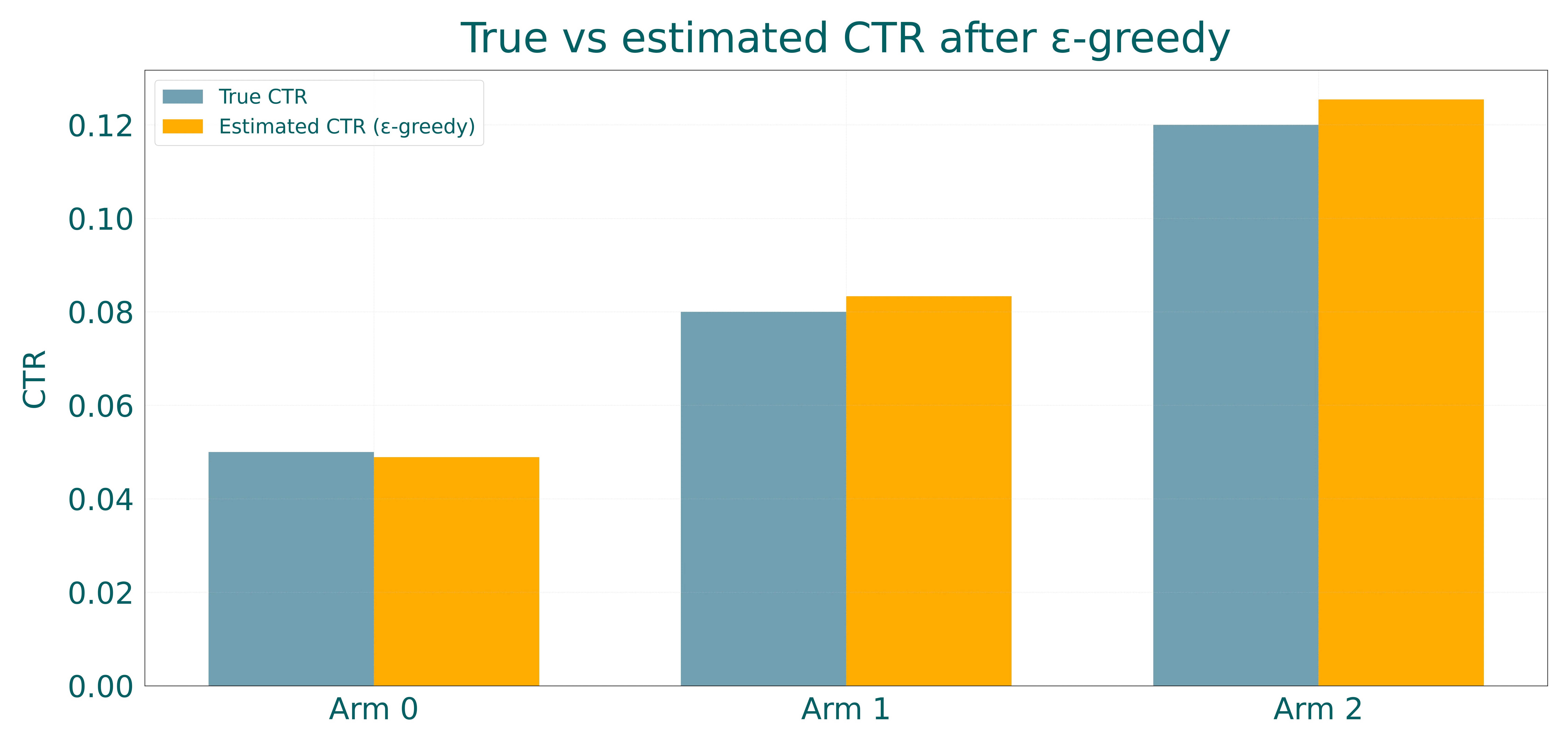
The estimate for the best arm is pretty close to its true CTR because it got sampled a ton. The weaker arms might be a bit noisier since they saw fewer samples, that’s a natural side effect of allocating traffic where it works.

Quick aside: if you read about bandits in academic papers, you’ll see a lot of talk about “regret”. Basically how much reward you left on the table compared to always playing the best arm from the start. That’s just (best_true_ctr * t) - cumulative_reward_t. The visualizations above already show ε-greedy reducing regret versus random, so we don’t need to get into formulas.

When do you use bandits vs classic A/B tests?

This isn’t really a silver bullet, it’s about what you’re optimizing for. Classic A/B testing makes sense when you want clean statistical inference and a crisp, defensible decision. You plan your sample size upfront, wait for the data to come in, then analyze it with your favorite statistical test. You accept that lots of users will see worse variants during the test. This is a good fit when you’re making high-stakes decisions about things you’ll keep for a long time, like your pricing page or core product flow. Bandits make sense when you care more about cumulative performance during the experiment itself. Traffic naturally shifts toward better options as evidence piles up. You’re not getting the same kind of “clean” fixed-horizon samples per arm, but you’re getting more clicks (or conversions or revenue) right now. This is great for always-on optimization problems, like rotating ad creatives in a feed or picking email subject lines for ongoing campaigns. Note that ε-greedy is the easiest algorithm to understand, but there are fancier ones like UCB and Thompson Sampling that often perform better. The core explore/exploit trade-off is the same, though.

Subscribe to the newsletter

We will only send you emails when new content is available

Email

Subscribe