What Implies Causation?
We’ve all heard the mantra: correlation does not imply causation. It’s true, and not remotely helpful when you’re the person who has to make a decision (ship a change, scale a campaign, or fund a feature). This post is a field guide to the opposite question: what does imply causation? I’ll skip the gatekeeping and walk through the designs, assumptions, and checks that turn “interesting correlation” into a causal claim you’d be comfortable defending in a meeting or retracting if the diagnostics say you’re fooling yourself.
The famous mantra that stalls us
Correlation does not imply causation.
This phrase seems to be very widely accepted among people and most people I talk to at least know the mantra. The phrase is so famous that it even has its own Wikipedia page. I did some research and couldn’t find the exact origin of the phrase, but it appears to have come from a book around 1880, but it’s so popular now that almost everyone knows about it. This has gotten to the point where the word “correlation” is almost seen as a bad word. It’s the quickest way to end a discussion. I’ve watched perfectly good ideas get thrown out because the word correlates sounds dirty, like you just confessed to p-hacking or manipulating the data.
However, whenever I hear this phrase, I can’t help but wonder if anyone knows what does actually imply causation. It’s clear that correlation does not, but what happens if we really want to determine causality? This phrase only tells me what not to do, but it doesn’t help me get any closer to the solution. We still have to make a call. Should we roll out the new onboarding? Will our new ad creative actually increase conversions? When I ask people, “what does imply causation?” I tend to get answered with very confused faces. So in this post I want to talk about the thing that actually implies causation; causal inference!
Definitions
-
Causality is the relationship between an event (the cause) and a second event (the effect), where the second event is understood as a consequence of the first. It’s the principle that one thing can influence another. The process of using data to determine causality is called causal inference.
-
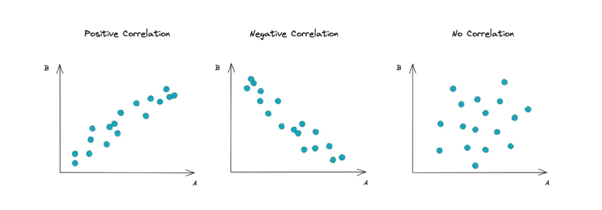
Correlation is a measure of how two variables are related to each other.
Correlation is helpful, but neither necessary nor sufficient
Why correlation isn’t sufficient
Three effects can produce correlations that aren’t causal:
- Confounding: an unobserved driver moves both your “cause” and your “effect.” E.g., seasonality increases both ad spend and revenue.
- Reverse causality: the arrow runs backward. Teams boost spend when revenue dips.
- Colliders: controlling for a common effect (like “users who saw any marketing”) can create a spurious relationship between independent causes.
Why correlation isn’t necessary
You can have a real causal effect with zero overall correlation if effects cancel out. Suppose a price change increases conversion for new users (+6pp) but decreases it for loyal users (-6pp), and your traffic mix is 50/50. True effects exist in each segment; the aggregate correlation goes to ~0. That doesn’t mean “no effect” it means “heterogeneous effects.”
What actually implies causation
To truly determine causality, we need to disentangle the relationship between a cause and its effect. This means isolating the effect of the cause from other factors that might influence the outcome. By doing so, we eliminate confounding and reverse causality, ensuring that any observed difference can be attributed to the cause itself. In principle, our goal is to observe the counterfactual, what would have happened if the cause had not been applied. For instance, if we want to know whether a new ad creative increases conversions, we would like to see what those same users would have done had they not seen the new ad. Since we cannot observe both realities for the same individual, the most powerful tool we have to approximate this counterfactual world is randomization. Randomization assigns individuals to a treatment or control group by chance, making the groups statistically equivalent on average. This allows us to compare their outcomes and infer whether the treatment had an effect. Randomization is therefore the gold standard for causal inference and when implemented in practice, it takes the form of a randomized controlled trial (RCT).
Randomized Controlled Trial (RCT)
An RCT is an experiment in which you randomly assign units (people, users, stores, etc.) to either receive a treatment or not, then measure outcomes in both groups. The “randomized” part is doing the heavy lifting: by flipping a coin (or running random.choice), you ensure that on average, the treatment and control groups are identical on every dimension like age, income, browsing history, coffee preference, etc. This means any systematic difference in outcomes can be attributed to the treatment itself, not to some lurking confounder.
The counterfactual logic
What we really want to know is: what would have happened to the treated group if they had not been treated? We can’t observe that (we either need time machines or identical twins with identical environments!). But randomization gives us the next best thing: a control group that looks exactly like the treatment group in expectation. The average outcome in the control group becomes our approximation for the counterfactual, and the difference between groups is the causal effect.
Why RCTs are the gold standard
Randomization does three powerful things:
- Eliminates confounding: Because assignment is random, there’s no systematic relationship between who gets treated and their potential outcomes. Seasonality, user quality, and any other confounder you can imagine are balanced across groups.
- No reverse causality: You control when and how treatment is applied. The treatment can’t be “caused” by the outcome.
- Simple inference: The math is clean. You can estimate the treatment effect with a difference in means, and standard errors follow directly from the randomization distribution.
This is why RCTs are considered the gold standard: if executed properly, they deliver causal estimates without requiring untestable assumptions about what you didn’t measure.
Example: A/B testing ad creative
Suppose your growth team wants to test a new ad creative. You randomly split incoming traffic: 50% sees the old creative (control), 50% sees the new one (treatment). You measure conversion rates over two weeks:
- Control: 2,000 users, 80 conversions → 4.0% conversion rate
- Treatment: 2,000 users, 100 conversions → 5.0% conversion rate
- Difference: +1.0 percentage point (pp)
Is that real? You run a two-sample proportion test and get . It’s suggestive but not quite significant at . You could have powered the test better (maybe you needed 3,000 per group for 80% power to detect a 1pp lift), or the effect might be smaller than you hoped. Either way, randomization ensures you’re not confusing “users who saw the new ad” with “users who arrived on a high-converting day.”
Example: Clinical drug trial
A pharmaceutical company wants to test a new blood pressure medication. They recruit 500 patients with hypertension and randomly assign 250 to receive the drug and 250 to receive a placebo (an inert pill that looks identical). Crucially, the trial is double-blind: neither the patients nor the doctors measuring blood pressure know who got the real drug. This eliminates placebo effects and experimenter bias.
After 12 weeks:
- Placebo group: average blood pressure reduction of 2 mmHg
- Drug group: average reduction of 8 mmHg
- Causal effect: 6 mmHg reduction attributable to the drug
Randomization ensures the groups were comparable at baseline (age, diet, exercise, baseline BP). The blinding ensures the measured difference isn’t driven by psychological effects or biased measurement. This is the design that gets drugs approved by regulatory agencies, and for good reason.
Example: No randomization
Let’s go back to the growth team’s example, but this time, you don’t randomize the treatment. Instead, you assign the new ad creative based on time of the day. In the morning you show the old creating and in the afternoon you show the new one. The problem is that you didn’t noticed that your traffic in the afternoon is a lot more qualified and aligned with your ICP (ideal customer profile) because it’s people coming back from work. That means that the new ad creative is more likely to convert in the afternoon than in the morning. This is a classic example of confounding.
Limitations of RCTs
RCTs are powerful, but they’re not always feasible or appropriate:
- Ethics: You can’t randomize people into smoking or poverty to measure health effects. If you believe a treatment is beneficial, withholding it from the control group may be unethical (though equipoise or genuine uncertainty often justifies trials).
- Cost and time: Running a large-scale RCT can be expensive and slow. A pharmaceutical trial might cost millions and take years. For fast-moving product decisions, you may not have that luxury.
- Interference: If units can affect each other (network effects, marketplace dynamics), randomization breaks down. Treating user A might change user B’s outcome even if B is in control. This is the “stable unit treatment value assumption” (SUTVA) violation, and it’s everywhere in platforms, marketplaces, and social networks.
- External validity: An RCT tells you the effect in your sample, under your conditions. It might not generalize to different populations, time periods, or contexts. A test that worked on your website in Q1 might fail in Q4.
- Compliance: People don’t always do what you randomize them to do. If 30% of the treatment group never uses the feature, your “intent-to-treat” estimate is diluted. You can estimate a “complier average causal effect,” but now you’re back to making assumptions.
When RCTs aren’t possible, we turn to quasi-experimental designs that try to approximate randomization using observational data and credible assumptions.
Quasi-experiments
When randomization isn’t an option because it’s too expensive, too slow, unethical, or just impossible, we turn to quasi-experimental methods. These designs leverage natural variation, policy quirks, or institutional rules to approximate the conditions of an RCT. The key difference: instead of creating randomness through coin flips, you find sources of variation that are plausibly “as-if random” and use them to isolate causal effects. You’re trading the certainty of randomization for the flexibility of observational data, which means you have to defend your assumptions more carefully.
Difference-in-Differences (DiD)
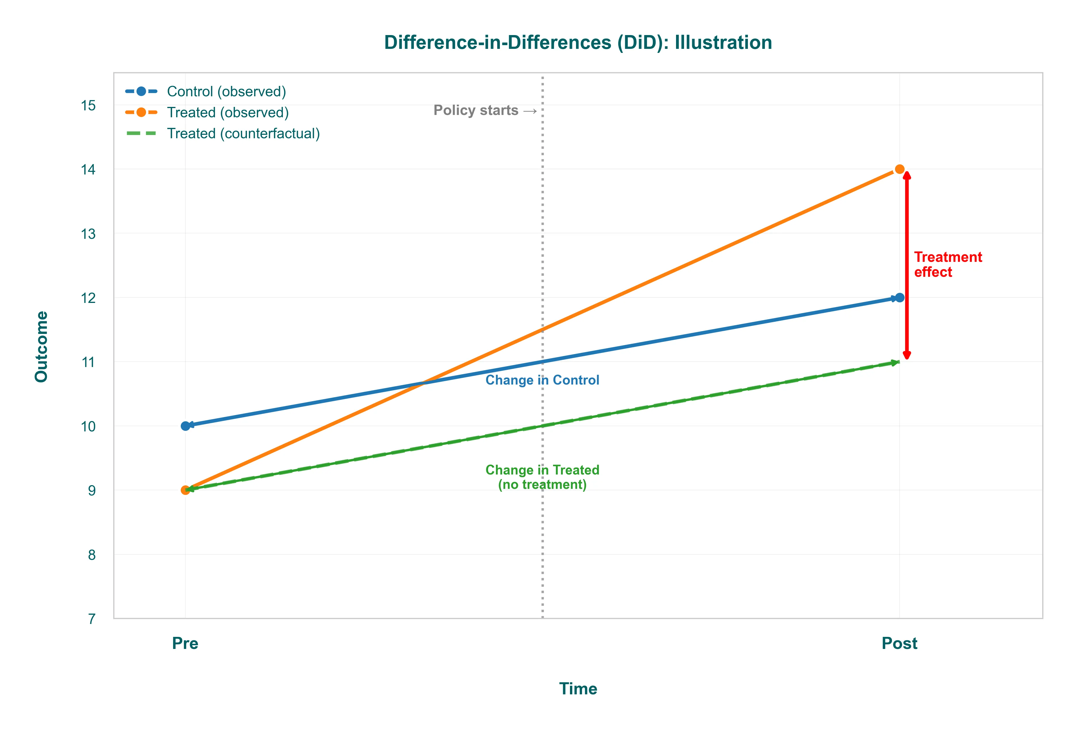
DiD is the workhorse when you have a treatment applied to one group but not another, and you observe both groups before and after the intervention. The intuition: compare how the treated group’s trend changed relative to a control group that wasn’t affected.
-
Example: Your company rolls out a new feature to users in the UK but not the US (maybe because of regulatory timing). You measure engagement for both groups before and after the UK launch. The treatment effect is the difference between the UK’s before-after change and the US’s before-after change. This “differences out” any time trend that would have happened anyway (seasonality, product updates that hit both markets).
-
Key assumption: Parallel trends. Absent treatment, the UK and US would have moved in parallel. You can’t test this directly post-treatment, but you can check pre-treatment trends: if they diverged before the launch, your DiD estimate is suspect. Plot those trends. If they wiggle together for six months and then split right when you launched, you have a decent case.
-
Common failure: Policy anticipation (users change behavior before treatment because they expect it) or a concurrent shock that only hits the treated group (a competitor launches in the UK the same week).
Regression Discontinuity (RDD)
RDD exploits a sharp cutoff: treatment is assigned based on whether a “running variable” crosses a threshold. If you can’t manipulate the cutoff precisely, and potential outcomes are smooth near the threshold, the people just above and just below are nearly identical (except for treatment status).
-
Example: A loyalty program gives a discount to customers who spend ≥ $500 in a quarter. You want to know if the discount causes higher retention. Compare customers who spent $490-$499 (no discount) to those who spent $500-$510 (got the discount). If spending is effectively continuous and customers aren’t bunching at $500 to game the system, this local comparison is as good as random assignment.
-
Key assumptions: No precise manipulation at the cutoff (check for bunching in a histogram of the running variable), and potential outcomes are smooth (use a flexible polynomial or local linear regression to avoid imposing functional form).
-
Common failure: People game the threshold (students retake a test to just pass; customers split transactions to hit $500), or you use too wide a bandwidth and end up comparing very different populations.
Instrumental Variables (IV)
IV is for when your treatment is endogenous (correlated with unobserved stuff that also affects the outcome) but you have an external “push” (the instrument) that shifts treatment without directly affecting the outcome. The instrument lets you isolate the causal part of the variation.
-
Example: You want to measure the effect of using a mobile app on purchase frequency, but app users are systematically different (more engaged, higher income). Your instrument: a push notification campaign that was sent to a randomly selected subset of users, encouraging them to download the app. The campaign affects app adoption (relevance), and it only affects purchases through app adoption (exclusion restriction). You use the campaign as an instrument to estimate the causal effect of app usage among the “compliers” (people who downloaded because of the notification).
-
Key assumptions: Relevance (instrument strongly predicts treatment; F-stat > 10 is a rough rule), Exclusion restriction (instrument affects outcome only through treatment; untestable but defendable with domain knowledge), Monotonicity (no “defiers” who do the opposite of what the instrument nudges).
-
Common failure: Weak instruments (relevance fails; your estimates blow up) or a hidden direct path (exclusion fails; maybe the notification itself reminds people to buy, independent of app usage).
When to use what
- DiD: You have pre/post data for treated and control groups, and you believe they would have trended together absent treatment.
- RDD: Treatment is assigned by a threshold you can’t manipulate, and you’re willing to estimate a local effect near the cutoff.
- IV: Treatment is endogenous, but you have an external push that shifts treatment and satisfies exclusion.
All of these designs require you to defend your assumptions. Plot your pre-trends. Check for bunching. Test instrument strength. Document the institutional details that make your “as-if random” claim credible. The rigor is in the diagnostics, not the method name.
Summary of causal inference designs
| Design | When to use | Core assumption | Typical failure |
|---|---|---|---|
| Randomized Controlled Trial (A/B test) | You can randomize exposure: product changes, pricing tests, emails, growth loops | Randomization breaks confounding; no interference; treatment is applied consistently | Peeking, novelty effects, noncompliance, sample imbalance |
| Natural Experiment | As-if random shocks: phased rollouts, policy thresholds, outages, lotteries | Assignment is unrelated to potential outcomes (as-if random) | “Shock” correlated with behavior (managers cherry-picked) |
| Difference-in-Differences (DiD) | Treated & control groups with before/after measurements | Parallel trends: absent treatment, the groups would have moved in parallel | Diverging pre-trends; policy anticipation |
| Regression Discontinuity (RDD) | Hard cutoff for treatment (score ≥ 70 gets discount) | No precise manipulation at the cutoff; smooth potential outcomes | Gaming the score; too-wide bandwidth |
| Instrumental Variables (IV) | You have a push that changes treatment but affects outcome only via treatment | Relevance (moves treatment), Exclusion (no direct path), Monotonicity (no “defiers”) | Weak instruments; hidden direct paths |
Conclusion
Correlation is a starting point, not an answer. It’s a blinking light that says “look here”. What does imply causation is a toolkit: randomized experiments when you can engineer them, quasi-experimental designs when the world hands you plausible variation, and a disciplined willingness to interrogate your assumptions at every step.
The methods we’ve covered like RCTs, DiD, RDD and IV are not just academic exercises. They’re the bridge between “this looks interesting” and “I’m confident enough to act on this.” They turn correlation into a defendable claim, or they force you to admit you don’t have one yet. That honesty is the point. Experiments fail. Pre-trends diverge. Instruments turn out to be weak. When that happens, you learn something: maybe your hypothesis was wrong, maybe your data aren’t rich enough, or maybe the world is more complicated than your model assumed. That’s not failure; that’s the scientific method doing its job.
Causal inference is messy, but it’s the best tool we have for turning data into decisions. So the next time someone invokes “correlation does not imply causation” to shut down a conversation, ask them: “Okay, so what would convince you?”.